Paged charts in Qlikview

Qlikview does not have a built-in paging mechanism for charts and tables. By paging, I mean returning a portion of the results (say top 5 salespeople), with "next" and "previous" buttons to view other portions - in the same way a web search with Google or Bing returns one page at a time.

To illustrate, this is a simple paged chart in Qlikview:
 

Here's how to do it.

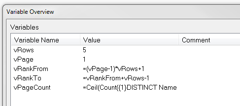
• Create the following variables
• vRows - contains the number of rows to display per page - 5 in this case
• vPage - the page number. Initialise to 1 for the first page.
• vRankFrom - the expression  =(vPage-1)*vRows+1
• vRankTo - the expression  =vRankFrom+vRows-1
• vPageCount - the expression  =Ceil(Count({1}DISTINCT Name)/vRows)
• Note the = sign on the three expressions
 



Set these variables

 
 
 
• Create 3 text boxes
• "Previous" or "<<"
• Lable the first one "<<" or "Prev" (or whtaver makes sense in your situation). 
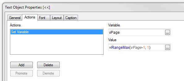
• Create a set variable action for vPage with the following expression:
  =RangeMax(vPage-1, 1).
  The RangeMax ensures that vPage will not be less than 1.
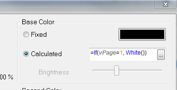
• Optionally set the font colour to black, and add the following calculate colour expression:
  =If(vPage=1, White())
  (Set to whatever colours you like to indicate active and disabled states)

• "Next" or ">>"
• As above, but use =RangeMin(vPage+1,vPageCount) for the vPage set variable action and =If(vPage>=vPageCount, White()) for the calculated colour expression.
• Page lable - this is a simple textbox displaying the expression:
  ='Page ' & vPage & ' of ' & Ceil(Count(Distinct Name) / vRows)
• Create the chart. We need a chart with some sort of ordering such as ranking salespeople by sales volumes. In the example the chart expression is simply Sum(Value), and we will sort by this value. The dimension is the field [Name]. To adapt it to work with the ranking, use the following calculated dimension to limit the values to the current page:
  
  =Aggr(If(Rank(Aggr(Sum(Value), Name)) >= vRankFrom And Rank(Aggr(Sum(Value), Name)) <= vRankTo, Name), Name)
  
  (The ranking functions wrap the chart expression (red) returning the dimension values (blue) that fall inside the range specified vt the vRankFrom and vRankTo variables). 
• On the sort tab, select Sort by "Y-value" descending.
• One the Presentation tab,  check the "Max Visible Number" box and enter the expression =vRows in the expression box.

Here is a QV document that implements the paging described above:

DataPaging.qvw

Action for previous button

Colour settings for previous button

Max Visible Number setting on Presentation tab

Handy data discovery tool

Here's a handy tool to assist in the early development and analysis of the data coming into your Qlikview documents.  There are three objects that you can copy from the attached Qlikview document and paste into your document. You do not need to modify your data model or load script in any way as these objects use standard QV built-in fuctionality.

• A tree-view list box with the tables and fields in your data model
• A text box containing summary statistics for the selected field (hidden until a field is selected)
• A dynamic list box containing the distinct values of the selected field (also hidden until a field is selected)

Here is a Qlikview document containing the 3 objects. Select a field name (any one) to make all three visible and copy from tis document into your Qlikview document.

Data Discovery.qvw

Creating the tools yourself

 If you are using QV Personal Edition, you will not be able to open the attached document, so here is how you can create these objects

The data structure listbox

Create a list box, select in the Field box, and enter the following expression:

=Aggr(Only({1} $Table) & '|' & Only({1} $Field), $Field, $Table)

Then check the "Show as TreeView" option and enter the vertical pipe "|" as the separator.

The text box

Create a text box, and add the following expression:

=Num(Count(Distinct [$(=$Field)]), '# ##0') & ' unique values
' & Num(Count([$(=$Field)]), '# ##0') & ' total values ('
 & Num(Count([$(=$Field)]) / (Count([$(=$Field)]) + NullCount([$(=$Field)])), '0%') & ')
' & Num(NullCount([$(=$Field)]), '# ##0') & ' null rows
' & Num(Count(If(Len([$(=$Field)])=0, [$(=$Field)])), '# ##0') & ' empty values'

On the Layout tab, add the following conditional expression:
Count($Field) = 1

The dynamic list box

Create a list box, select and add the expression:
=[$(=$Field)]

On the Layout tab, add the following conditional expression:
Count($Field) = 1

Conclusion

Remember to select a field in the data discovery list box to see the other two objects. Feel free to use and modify the objects in any way you please. With all the usual disclaimers...